Backup

Shows how to backup data.

import dman
from dman.numeric import carray, barray
from dman.plotting import PdfFigure

import numpy as np
import matplotlib.pyplot as plt
import warnings


@dman.modelclass(compact=True, storable=True)
class Config:
    degrees: carray[int]


@dman.modelclass(storable=True, store_by_field=True)
class Experiment:
    x: barray = dman.recordfield(subdir='samples')
    y: barray = dman.recordfield(subdir='samples')
    z: dman.mruns
    fig: PdfFigure = None


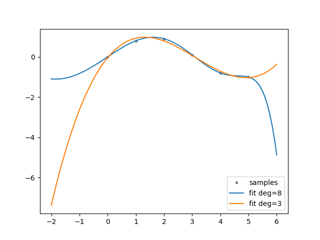
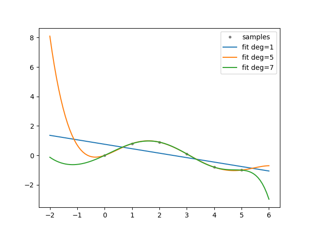
def experiment(cfg: Config):
    """Generate experiment data.
    Based on: https://numpy.org/doc/stable/reference/generated/numpy.polyfit.html.
    """
    xp = np.linspace(-2, 6, 100)
    x = np.array([0.0, 1.0, 2.0, 3.0, 4.0, 5.0])
    y = np.array([0.0, 0.8, 0.9, 0.1, -0.8, -1.0])
    z = dman.mruns(stem="poly", store_subdir=False, subdir='fit')

    fig, ax = plt.subplots(1, 1)
    ax.plot(x, y, ".", color="gray", label="samples")
    for d in dman.tui.progress(cfg.degrees, description="order"):
        with warnings.catch_warnings():
            warnings.simplefilter("ignore", np.RankWarning)
            zz = np.polyfit(x, y, d)
        z.append(zz.view(barray))
        p = np.poly1d(zz)
        ax.plot(xp, p(xp), "-", label=f"fit deg={d}")
    ax.legend()
    return Experiment(x, y, z, PdfFigure(fig))


def evaluate(cfg: Config):
    """Evaluate the provided configuration.
    Store a backup of the last executed experiment.
    """
    current = dman.load('current', default=None)
    if current is not None:
        with dman.track("__backup__", default_factory=dman.mruns_factory(stem='backup')) as reg:
            reg: dman.mruns = reg  # for type hinting
            reg.append(current)
    current = experiment(cfg)
    dman.clean('current')       # clear old current
    dman.save('current', current)
    return current

# Clear the backed up runs if they exist (for a fresh start)
dman.clean('__backup__')
dman.clean('current')

# Execute several configurations
res1 = evaluate(Config([1, 5, 7]))
res2 = evaluate(Config([8, 3]))
res3 = evaluate(Config([1, 5, 7]))

• 
• 
• 

order [3/3] ━━━━━━━━━━━━━━━━━━━━━━━━━━━━━━━━━━━━━━━━ 100% 0:00:00
order [2/2] ━━━━━━━━━━━━━━━━━━━━━━━━━━━━━━━━━━━━━━━━ 100% 0:00:00
order [3/3] ━━━━━━━━━━━━━━━━━━━━━━━━━━━━━━━━━━━━━━━━ 100% 0:00:00

We can examine the results and see that they are correct.

dman.tui.pprint(res1)

Experiment(
│   z=[barray([-0.30285714,  0.75714286]), barray([-8.33333333e-03,  1.25000000e-01, -5.75000000e-01,
│   │    6.25000000e-01,  6.33333333e-01,  1.40925649e-14]), barray([-1.91046771e-04,  8.51553918e-04,  5.63990582e-03,
│   │   -3.21702635e-03, -1.74163595e-01,  9.60491579e-02,
│   │    8.75031051e-01, -7.25194643e-16])],
│   fig=<dman.plotting.PdfFigure object at 0x7fe4a1d6eda0>
)

The file structure is then as follows. Note that a pdf has been created for each experiment containing the produced figures. Feel free to take a look.

dman.tui.walk_directory(dman.mount())

📂 .dman/cache/examples:patterns:example2_backup
┣━━ 📂 __backup__
┃   ┣━━ 📂 backup-0
┃   ┃   ┣━━ 📂 fit
┃   ┃   ┃   ┣━━ 📄 poly-0.npy (144 bytes)
┃   ┃   ┃   ┣━━ 📄 poly-1.npy (176 bytes)
┃   ┃   ┃   ┗━━ 📄 poly-2.npy (192 bytes)
┃   ┃   ┣━━ 📂 samples
┃   ┃   ┃   ┣━━ 📄 x.npy (176 bytes)
┃   ┃   ┃   ┗━━ 📄 y.npy (176 bytes)
┃   ┃   ┣━━ 📄 backup.json (1.5 kB)
┃   ┃   ┗━━ 📄 fig.pdf (14.3 kB)
┃   ┣━━ 📂 backup-1
┃   ┃   ┣━━ 📂 fit
┃   ┃   ┃   ┣━━ 📄 poly-0.npy (200 bytes)
┃   ┃   ┃   ┗━━ 📄 poly-1.npy (160 bytes)
┃   ┃   ┣━━ 📂 samples
┃   ┃   ┃   ┣━━ 📄 x.npy (176 bytes)
┃   ┃   ┃   ┗━━ 📄 y.npy (176 bytes)
┃   ┃   ┣━━ 📄 backup.json (1.3 kB)
┃   ┃   ┗━━ 📄 fig.pdf (13.3 kB)
┃   ┗━━ 📄 __backup__.json (597 bytes)
┗━━ 📂 current
    ┣━━ 📂 fit
    ┃   ┣━━ 📄 poly-0.npy (144 bytes)
    ┃   ┣━━ 📄 poly-1.npy (176 bytes)
    ┃   ┗━━ 📄 poly-2.npy (192 bytes)
    ┣━━ 📂 samples
    ┃   ┣━━ 📄 x.npy (176 bytes)
    ┃   ┗━━ 📄 y.npy (176 bytes)
    ┣━━ 📄 current.json (1.8 kB)
    ┗━━ 📄 fig.pdf (14.3 kB)